Lab 10

Preview

In this lab, we use a Bayes filter to tackle grid localization. Essentially, this filter uses various inputs from datapoints it collects, as well as control inputs on what we command the robot to do, and a prior belief of its position to determine where it thinks the robot is. By knowing the environment the robot is in, we can calculate our belief of where our robot might plausibly be within the map that best matches the data we have been given. In layman's terms, this approach has the robot look around in its environment. Then, it can compare these observations to what best matches it given the room where the robot is in.

Approach

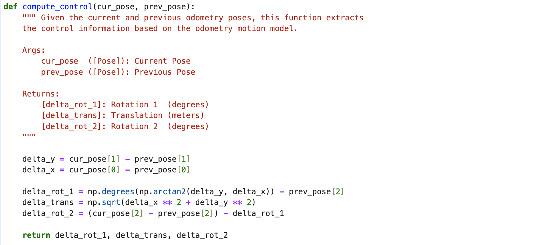
The code for this lab is split into several key sections. First, we must actually collect the data to use for our filter. In our iterative processs, we always start with some belief matrix of how likely we think the robot is to be at every position. Note that this matrix is actually 3D, even though the robot is in a 2D environment, with our third axis representing orientation. Notice that with this approach, the precision of our estimate is only as good as the granularity of our matrix. The more memory we dedicate to it, the more smaller the intervals between matrix cells, sacrificing memory for accuracy. Anyways, our first function needs to compute the transformations applied to our robot. That is, given the current and previous pose, come up with a series of a rotation, followed by a transltion and then another rotation, that should be equivalent to the appropriate change in position. You can see the code below. Overall, the approach first gets the difference on the X and Y axes. Using this, we can calculate the angle between the two points, and subtract our previous angle from it (to turn our robot in that direction). Our translation magnitude is simply the distance, and for the second roation, we basically do the same thing and back calculate how much to turn to match the given orientation.

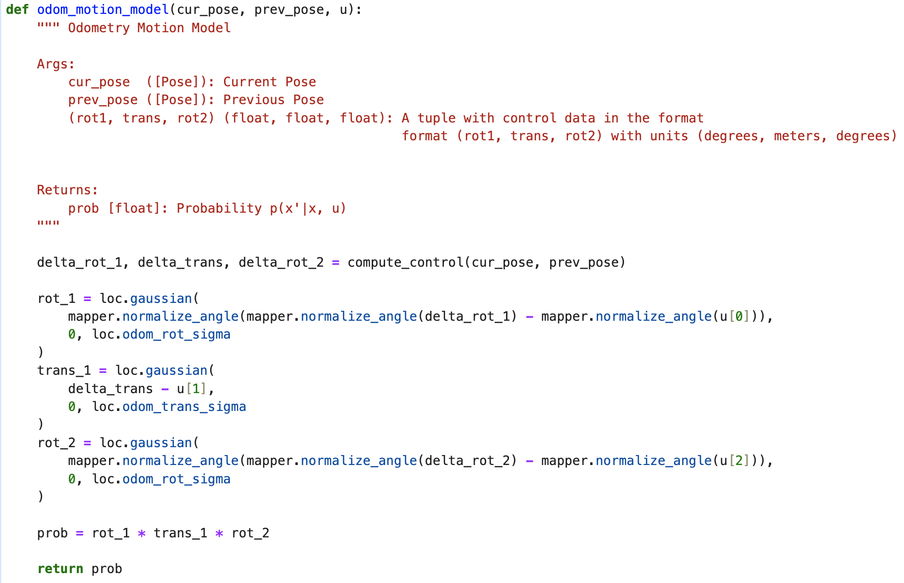
The second part of the code gets the the new probabilities given an action we want our robot to perform, which is basically a sequence of the rotation and translation and second rotation from the previous function. We model each of these as a gaussian, and multiply them together, assuming that each of the equivalent actions are independent. In the real world, this may not be exactly true, like with imperfections with motor turning or for other reasons, but is a pretty reasonable assumption to make in simulation. The final product then is the distribution of the final state after all actions have been done. You can see the code below.

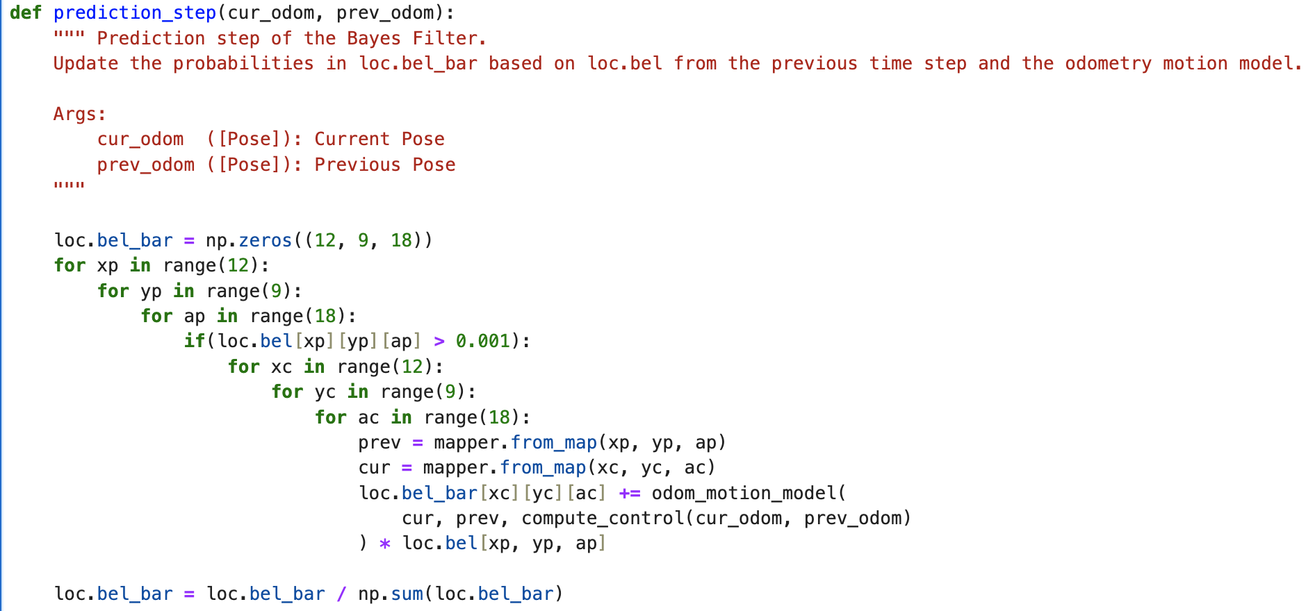
The third step is putting it all together! Using the control implied from the previous and current odomoetry provided, we can update our bel values. We do this update across all elements of the previous, and then current matrix. This calculates a new belief matrix we normalize and then return. To speed this part up, I chose to ignore value with small probability to speed things up, at the expense of precision.

The fourth step is pretty simple. Mimicking the sensor behavior described, we calculate a gaussian for the results returned by the sensor across all 18 measurements we take, to get the final part of the equation for the filter.

Finally, the fifth step implements the full filter for one step. For all of the current positons, we calculate our belief matrix using the updates we get from our sensor model in the previous step. Mulitplying this with each grid location yields the probability of each position being where our robot actually is. Normalizing this, we can find the largest probability value to estimate our location in the grid.

Results

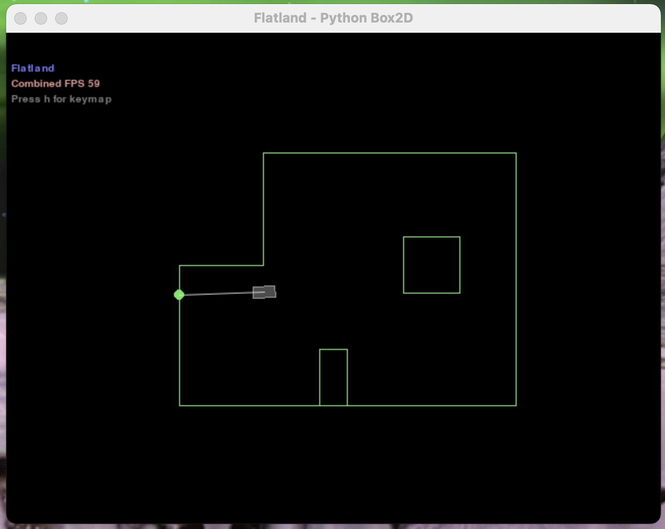
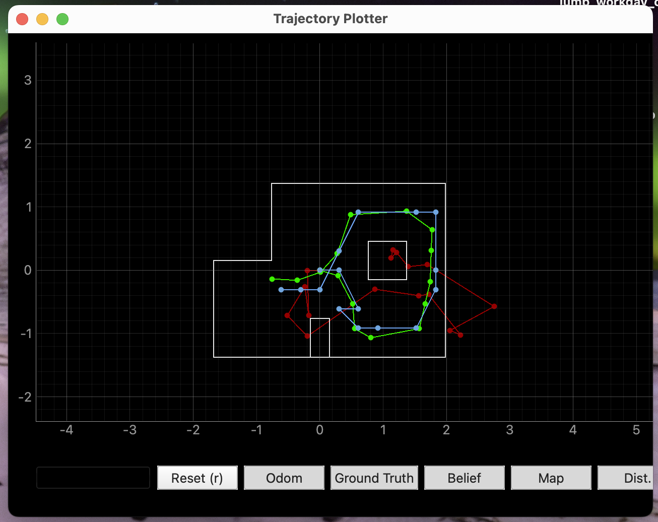
Overall, the results of this project turned out pretty well considering how fast it runs; see the images included below. Primarily due to the optimization I made to discard low probability grid locations in the predictions step, our model is not as accurate as it could be, but it runs in under 20 seconds. However, even if this were fixed, there would still be some limitations. Although the bayes filter can be a really good tool for localization, it struggles with terrain that is not very distinguishable. In layman's terms, this approach, which compares the surroundings a robot sees with what it might expect to see at any given location on a map, does not do very well when the robot cannot see clear identifiable landmarks. In fact, it might even perform much worse if the terrain is actively difficult to distinguish, like in a maze. You can see that here where the estimates are a little bit off when the robot is in a somewhat symmetrical position. But overall, it still managed to do quite well, and I am happy with my accomplishment in this lab.